Chapter 2 Aligning Sequence Data

2.1 What is an alignment ?

In biology, comparison is at the heart of many studies: between individuals, between species, between sequencing runs, etc… In order to do this at a fine-grained level and extract knowledge from it, we need to compare what is comparable, this is where sequence alignment steps in. In broad terms, during sequence alignment, we aim to find regions similar to each other in two or more sequences and group them together. When this process is done with only two sequences it is called a pairwise alignment. When three or more sequences are used it is called multiple alignment. We will first focus on pairwise alignment as it is used as the basis for the more complex multiple alignment.

2.1.1 Why align ?

The first question we might ask ourselves is why align at all? If we want to compare two sequences there are plenty of distances and metrics out there to use. Something like the Hamming distance¹²⁸ is very quick and easy to compute by comparing characters two by two. It is however ill-suited to our needs in biology: it can handle substitutions but indels induce very large Hamming distances. Indeed, insertions and/or deletions shift one of the sequences, compared to the other, and introduce many character-to-character differences that could be explained by a single indel.

For example, let us consider the two following sequences: ATGTGCAGTA and AGTGCAGTAC. if we count the differences character by character, except the first pair of A, all the characters are different (c.f. below). However, if we consider that the first T was deleted and a C was inserted at the end of the second sequence then we can see that none of the characters are actually different. In order to represent insertions and deletions gaps are inserted in the sequences as seen below:

ATGTGCAGTA-
A-GTGCAGTAC

This problem of comparing two sequences with insertions or deletions is a fairly well-studied one in text algorithmics: the string-edit problem¹²⁹. Some metrics like the Levenshtein distance¹³⁰ and the edit distance¹²⁹ exist and are closely related to the pairwise sequence alignment problem, finding the minimal number of substitution, insertion of deletion operations to go from one sequence to the other.

Sequence alignments have many downstream uses. They are the basis of comparative genomics¹³¹ and are used to infer evolutionary relationships, phylogenetic tree reconstruction methods usually take multiple sequence alignments as input^132–136. Sequence alignments have been used to study protein structure^137,138 and function^139,140. They can be used to correct sequencing errors^82,84,141 or detect structural variations in genomes^142,143. All this to say that they are absolutely fundamental to the field of computational biology and errors in alignments can lead to errors somewhere down the line.

2.1.2 How to align two sequences ?

There are two approaches for pairwise alignment¹⁴⁴: global alignment, where the entirety of both sequences is used, and local alignment, where we only seek to find regions in each sequence that are most similar to each other. Global alignment is used when the two sequences are expected to be quite similar (e.g. comparing two related proteins), whereas local alignment is mostly used when we expect the sequences to be fairly different but with highly similar regions, like genomes of two distantly related species that share a highly conserved region.

The seminal method for global pairwise alignment was the Needleman-Wünsch algorithm¹⁴⁵ based on a dynamic programming method. A decade later, the Smith-Waterman algorithm¹⁴⁶ was developed with similar ideas to perform local alignment. Both are still used today for pairwise alignment.

Dynamic programming is often used to solve complex problems by breaking it into smaller sub-problems and solving each one optimally and separately^147,148, it is particularly useful when we wish to have a precise alignment between 2 sequences.

2.1.2.1 Global alignment

The fundamental algorithm for globally aligning two sequences is the Needleman-Wünsch (NW) algorithm¹⁴⁵. The goal is finding the alignment with 1) the lowest edit-distance or 2) the highest alignment score. These two are equivalent so in this section we will maximize the alignment score.

The first thing we need to know is how to compute a score on a given alignment. To do this, we assign costs to each operation. Usually matches (i.e. aligning two identical characters) are given a positive cost and mismatches or indels a negative cost. If we assign a cost of +1 to a match and a cost of -1 to mismatches and indels then the alignment presented above in Section 2.1.1 would have an alignment score of 9 - 2 = 7 (9 matches and two indels).

The NW algorithm is based on a simple recurrence relation: the optimal alignment score of two sequences \(S_1\) and \(S_2\) of lengths \(n\) and \(m\) respectively is the maximum of:

1. The optimal alignment score of \(S_1[1,n-1]\)⁴ and \(S_2[1,m-1]\) plus the cost of a match or mismatch between the \(n^{th}\) character of \(S_1\) and the \(m^{th}\) character of \(S_2\)

2. The optimal alignment score of \(S_1\) and \(S_2[1,m-1]\) plus the cost of an indel

3. The optimal alignment score of \(S_1[1,n-1]\) and \(S_2\) plus the cost of an indel

This simple relation can be used to compute optimal global alignment score for two sequences. However, if it is implemented naively it can be very inefficient as the number of scores to compute grows exponentially with sequence lengths, and many intermediary alignment scores need to be computed many times. This is where dynamic programming comes in: these intermediary costs are pre-computed in an efficient manner and one can then deduce the optimal alignment from these. This pre-computing step is usually represented as filling out a matrix, whose rows and columns represent the characters in each sequence to be aligned, with partial alignment scores.

If \(S_1\) represents the rows of the matrix, and \(S_2\) the columns, the value \(C(i,j)\) of a cell \((i,j)\) of this matrix represents the optimal alignment score between \(S_1[1,i]\) and \(S_2[1,j]\). In the recurrence relation described above the alignment score as dependent on the optimal alignment scores of subsequences, when filling out the dynamic programming matrix we proceed in the inverse fashion by using the scores of short subsequences to build up the scores of progressively longer sequences.

We will go here through a short example showing how the NW algorithm is used to align two short sequences: \(S_1=\)ACCTGA and \(S_2=\)ACGGA. The first step is to represent the dynamic programming matrix, prefix each sequence with an empty character and label the rows of the matrix with one of the sequences and the columns with the other (this extra row and column at the beginning of each sequence are indexed as column and row 0). In this matrix, due to the recurrence relation stated above, the score of a particular cell, \(C(i,j)\), is the maximum of:

1. The score in the diagonally adjacent cell \(C(i-1,j-1)\) plus the cost of a match or mismatch between \(S_1[i]\) and \(S_2[j]\).
2. The score of the cell to the left \(C(i,j-1)\) plus the cost of an indel
3. The score of the cell on top \(C(i-1,j)\) plus the cost of an indel

Therefore, in order to compute \(C(i,j)\) we need to know the three values of \(C(i-1,j-1)\), \(C(i-1,j)\) and \(C(i,j-1)\). This is the reason why we start with an extra column and row at the beginning of each sequence that we can fill out with the increasing costs of indels. In our case since the cost of an indel is -1, this row and column are filled out with decreasing relative integers, as can be seen in Figure 2.1A.

From this starting point we can fill out the dynamic programming matrix with all the alignment scores. To compute \(C(1,1)\) we have three possible values:

1. \(C(0,0)\) plus the cost of a match between \(S_1[1]=A\) and \(S_2[1]=A\): \(0+1=1\)
2. \(C(0,1)\) plus the cost of an indel: \(-1 -1 = -2\)
3. \(C(0,1)\) plus the cost of an indel: \(-1-1=-2\)

By taking the maximum out of these three values we can fill out the matrix cell with \(C(1,1)=1\). By continuing this process until we fill out the whole matrix we obtain the scores visible in Figure 2.1A. This is enough if we only want to compute the optimal global alignment score between \(S_1\) and \(S_2\), contained in cell \((n,m)\). If we want to deduce the operations leading to it, and therefore the alignment itself, we need to keep track of which operation we made to get a specific score. The easiest way to do that is to also consider this matrix as a graph where each cell is a vertex. When we compute the score of cell \((i,j)\) we add an edge from this cell to the previous cell that was used to compute \(C(i,j)\). In our example above, we obtained \(C(1,1)\) from a match and \(C(0,0)\), so we can add an edge in our graph going from cell \((1,1)\) to cell \((0,0)\). The filled out matrix with the graph edges represented as arrows can be seen in Figure 2.1B.

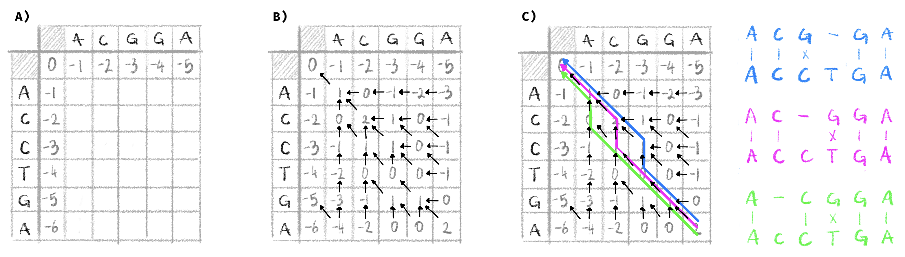
Figure 2.1: Example global alignment with the Needleman-Wunsch algorithm.
This figure represents three different steps in the NW algorithm, with a match cost of +1, a mismatch cost of -1 and an indel cost of -1. A) the matrix is initialized with \(S_1\) as the columns and \(S_2\) as the rows. Column and row 0 are filled out. B) The dynamic programming matrix is filled out, and the alignment graph is constructed. C) The alignment graph is traversed from the vertex in the bottom right cell to the vertex in the top left cell. Each of the three possible paths corresponds to an optimal global alignment, represented on the right.

Once this matrix (and corresponding graph) is filled out, we can deduce the alignment by following a path through the graph starting at cell \((n,m)\) to cell \((0,0)\). A diagonal edge starting at \((i,j)\) indicates a match or mismatch between \(S_1[i]\) and \(S_2[j]\), a vertical edge indicates a gap in \(S_2\) and a horizontal edge a gap in \(S_1\). This can lead to several optimal alignments if there are several such paths in the graph. In our case, this algorithm yields three equally optimal global alignments shown in Figure 2.1C.

This algorithm although guaranteed to result in an optimal alignment, has a time complexity of \(\mathcal{O}(nm)\) where \(n\) and \(m\) are the lengths of the sequences to align¹⁴⁴. Some methods have been proposed to speed up¹⁴⁹, however the complexity is still \(\mathcal{O}(nm/\log(n))\). Lower bounds have been studied and there is not much optimization to be done if optimal exact alignment is needed^150,151. If we want to do better we have to rely on heuristics.

Another issue is space complexity since we need to store the matrix, the space complexity is also \(\mathcal{O}(nm)\). If we wish to align 2 human genomes we would need to store \(\approx 10^{19}\) matrix cells, which would amount to 10 Exabytes of storage (i.e. the storage scale of a data-center) if we use 8bit integers. However, in practice, we can do much better than that, and construct an optimal alignment in linear space complexity \(\mathcal{O}(n+m)\)¹⁵² meaning we would only need a couple gigabytes to store the matrix for 2 human genomes. This resulted in an improved global alignment algorithm, the Myers-Miller algorithm¹⁵³, implemented in the EMBOSS stretcher alignment software¹⁵⁴.

2.1.2.2 Local alignment

In global alignment two full sequences are aligned to each other. In local alignment the goal is to find the optimal alignment of two subsequences from these parent sequences. The main algorithm for locally aligning is the Smith-Waterman (SW) algorithm¹⁴⁶, developed a decade later than NW.

The two algorithms are very similar, SW also relies on first building the dynamic programming matrix with the same parametrizable costs for matches, mismatches and indels as NW. One key difference is that the optimal scores in the matrix are bound by 0 so they cannot become negative. We only store edges in the alignment graph if the starting cell has an alignment score > 0.

In this new formulation, the score in cell \(C(i,j)\) is the maximum of the following values:

1. The score in the diagonally adjacent cell \(C(i-1,j-1)\) plus the cost of a match or mismatch between \(S_1[i]\) and \(S_2[j]\).
2. The score of the cell to the left \(C(i,j-1)\) plus the cost of an indel.
3. The score of the cell on top \(C(i-1,j)\) plus the cost of an indel.
4. \(0\).

If we use the SW algorithm to locally align the two example sequences \(S_1\) and \(S_2\) and the same costs as used above, we obtain the dynamic programming matrix and graph shown in Figure 2.2.

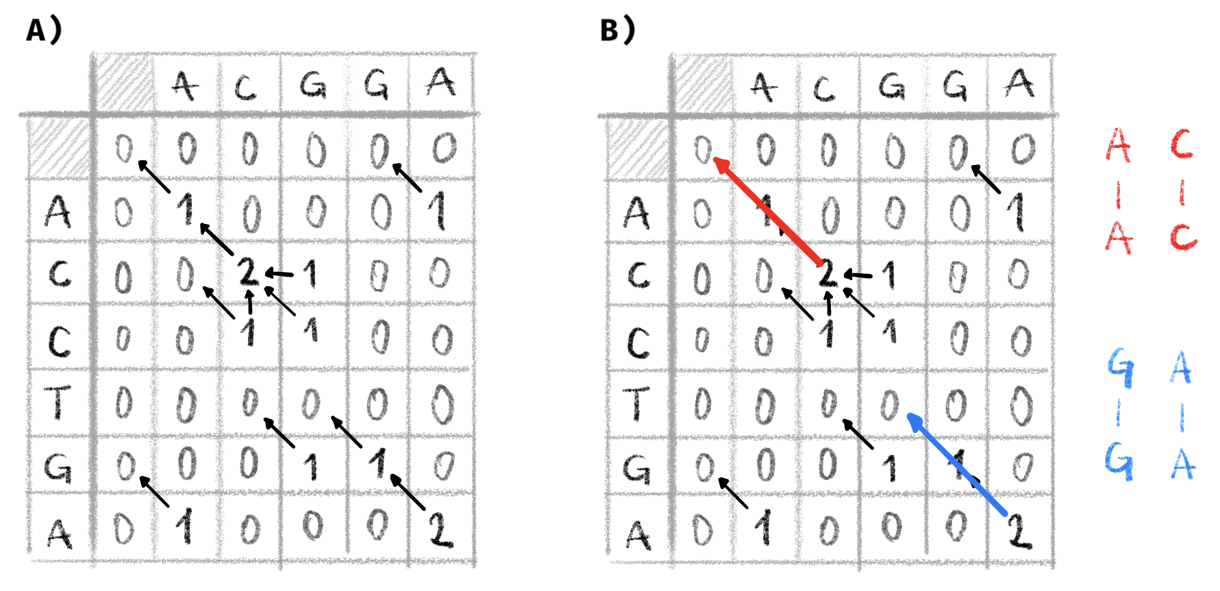
Figure 2.2: Example local alignment with the Smith-Waterman algorithm.
Two sequences \(S_1\) and \(S_2\) (the same as in Figure 2.1) are locally aligned. A match has a cost of +1, a mismatch a cost of -1 and indels a cost of -1. A) The dynamic programming matrix is filled out and the alignment graph constructed. Alignment scores are constrained to be non-negative. B) We find paths in the graph between the vertex with the maximal score and one with a score of 0. Here there are two such paths resulting in two optimal local alignments represented on the right.

The traceback part to determine the optimal alignment is very similar to NW, however instead of starting at cell \((n,m)\), we start at the cell in with the maximal alignment score and follow the path back until we arrive at a cell with an alignment score of 0. In the example shown in Figure 2.2, two cells contain the maximal alignment score of 2. Tracing back from these cells gives two optimal local alignments between \(S_1\) and \(S_2\): AC to AC and GA to GA.

Since the SW algorithm is so similar to NW it has the same quadratic time and space complexity. However, the same optimization can be used to bring it down to a linear space complexity¹⁴⁴. These optimizations resulted in the Huang and Miller algorithm¹⁵⁵, implemented in the EMBOSS Lalign tool¹⁵⁴, and the Waterman Eggert algorithm¹⁵⁶.

Both the NW and the SW algorithms are implemented in many different software tools and are used widely to perform pairwise alignments of short sequences^154,157,158. Some versions even benefit from hardware acceleration with version implemented for specific CPU instruction sets¹⁵⁹ or GPUs¹⁶⁰ to substantially speed up alignment.

2.1.3 Scoring and substitution models

In the examples used above to present the NW and SW algorithms, we used a very simple cost function: a match has a cost of +1 while mismatches and indels have a cost of -1. This is really the simplest cost function we can use but also the crudest. In many cases it may be interesting to infuse this cost function with biological knowledge. For example some substitutions occur more rarely than others in nature so it would stand to reason to penalize those more than other, more common, substitutions.

These biology-aware cost functions usually take the form of a matrix, called scoring or substitution matrix, often corresponding to an underlying evolutionary model. When using these matrices, matches and mismatches between specific characters are given. For example the cost of aligning an A and a G might be lower than aligning that same A with a T. A lot of different substitution matrices have been developed especially for protein alignments¹⁶¹, developed with different techniques and underlying models and with different intended applications.

The earliest and simplest substitution matrices are match/mismatch matrices. They are effectively what we used above, where all matches are given a fixed positive score and all mismatches a fixed negative score. In our examples above the corresponding substitution matrix would be a four by four matrix with ones on the diagonal indicating matches and -1 everywhere else. These are simple and useful, but when dealing with proteins, they have a severe limitation as they ignore the biology of amino acids.

In order to reflect this biological reality of proteins, new substitution matrices were developed using Log-odds models based on the fact that substitutions in amino acids are not equiprobable, and some mutations between related amino acids (e.g. I and L) are much more common than others. Two of the most widely used substitution matrices, PAM and BLOSUM matrices, were built this way. The score for aligning residue \(i\) with residue \(j\) is given by the matrix entry \(S_{ij}\) by looking at the background frequencies (i.e. how often one expects to see a particular residue in a sequence) of \(i\) and \(j\) denoted \(p_i\) and \(p_j\) respectively and the frequency \(q_{ij}\) with which \(i\) and \(j\) are aligned in accurate biological alignments. With these values we can compute the substitution score \(s_{ij}\) as a Log-odds¹⁶¹:

\[ S_{i,j}=\log\bigg(\frac{q_{ij}}{p_ip_j}\bigg) \]

This Log-odds formulation yields values with nice properties for sequence alignment. \(q_{ij}\) can be thought of as the probability of the alignment between amino acids \(i\) and \(j\) resulting from a substitution, and \(p_ip_j\) is the probability under the null hypothesis that both of these amino acids were aligned randomly. Therefore the log of the ratio is negative when the random alignment is more frequent (meaning the substitution is unlikely), and positive when the substitution is likely. Both \(p_i\) and \(p_j\) are easy to compute from available biological sequence data, the real work in developing a Log-odds based substitution matrix is to estimate \(q_{ij}\) values, and that is often done using biologically accurate protein sequence alignments.

The PAM matrix, developed in 1978¹⁶², is one such matrix. A point accepted mutation (PAM) is defined as the substitution of one amino acid by another that is accepted by natural selection (i.e. visible along the branch of a phylogenetic tree). Dayhoff et al. also defined a PAM as an evolutionary distance, where two sequences distant by one PAM are expected to have one amino acid substitution per one hundred residues, which is equivalent to expecting a substitution at 1% of positions. To develop their matrix, Dayhoff et al. used phylogenetic trees built on 71 families of closely related proteins and counted the PAMs that appeared in these trees. This resulted in a matrix \(A\) where \(A_{ij}=A_{ji}=\) the number of times a substitution between amino acids \(i\) and \(j\) was observed in the trees. By using trees built on closely related sequences, Dayhoff et al. could be fairly certain that the observed substitutions were the result of a single mutation and not many subsequent mutations over long evolutionary times. From this matrix \(A\), Dayhoff et al. reconstructed the mutation probability \(M_1\) where entries \(M_{1,ij}\) represent the probability of amino acid \(j\) being replaced by amino acid \(i\) after an interval of 1 PAM. Entries of this matrix are computed as follows:

\[\begin{align} M_{1,ij}&=\frac{\lambda m_j A_{ij}}{\sum_i A_{ij}}\;\; & \text{if}\;\;i\neq j\\ M_{1,ij}&=1-\lambda m_j & \text{if}\;\; i = j \end{align}\]

here \(m_j\) is the observed mutability of amino acid \(j\), and \(\lambda\) is a constant factor used to tune the matrix so that it reflects mutation rates corresponding to 1 PAM where 99% of positions are unchanged, which means that the diagonal of \(M_1\) must sum to 0.99. By assuming that evolution follows a Markov process it is simple to derive the mutation matrices for sequences separated by greater evolutionary distances. The \(M_n\) matrix, corresponding to a distance of \(n\) PAMs is equal to \(M_1^n\). Finally the \(q_{ij}\) values can be derived with \(q_{ij}=p_jM_{ij}\). By choosing different values of \(n\) for the mutation matrix we can estimate scoring matrices for sequences that are at varying evolutionary distances from one another. The correspondence between PAMs and the observed proportion of different residues is not one to one, therefore a distance of 250 PAMs corresponds to around only about 20% of identical residues where a distance of 180 PAMs corresponds to around 27% identical residues^161,162. Therefore the PAM₂₅₀ matrix, derived from \(M_{250}\), is suited to align more distantly related proteins than the PAM₁₈₀ for example. By changing the mathematical model underlying the estimate of mutation probabilities, PAM-like matrices¹⁶³ were later developed based on the same principles.

The other main type of substitution matrix is the BLOSUM matrix (Block Substitution matrix), developed in 1992¹⁶⁴. Instead of using whole, closely-related, protein sequences like the PAM matrices, the values of \(q_{ij}\) were estimated on highly conserved segments, called blocks, across whole protein families. The \(q_{ij}\) values are then estimated as the number of time amino acids \(i\) and \(j\) are aligned divided by the number of total amino acid pairs in the alignment. Therefore \(q_{ij}\) is the observed frequency of the aligned pair of amino acids \(i\) and \(j\) in all the conserved blocks. As with PAM matrices, several BLOSUM matrices were constructed, designed for aligning sequences with different evolutionary distances. The BLOSUM62 matrix was estimated on blocks in aligned sequences that are at most 62% identical, BLOSUM80 on sequences that are at most 80% identical. Therefore, inversely to the PAM matrices, the higher the number of the BLOSUM matrix the more suited it is to align more closely related sequences.

PAM and BLOSUM matrices have fairly broad use-cases and are widely used in alignment. However, many other protein substitution models exist. Instead of using log-odds, some substitution models were developed by estimating scores with maximum-likelihood approaches^165,166. Some matrices were developed with very specific usage conditions in mind, tailored to specific types of proteins like transmembrane^167,168, disordered¹⁶⁹ or polar/non-polar¹⁷⁰ proteins. Some matrices were developed to align sequences from specific organisms like P. falciparum¹⁷¹ (responsible for malaria) or HIV¹⁷². A substitution matrix was even developed in 2005 specifically for global rather than local alignment¹⁷³.

This wealth of protein substitution matrices reflects the biological and evolutionary diversity of proteins, however substitution matrices for aligning DNA sequences are much less common. Some work has been done to derive matrices similar to PAM matrices from DNA alignments¹⁷⁴. Codon substitution matrices^175,176 have been developed as well, although they are used in DNA sequence alignment, ultimately they use knowledge derived from protein alignments.

2.1.4 Dealing with gaps

In the NW and SW examples of Section 2.1.2, as with the simplistic match/mismatch costs, we used a very simple cost of insertions and deletions: any indel has a cost of -1. As was the case with substitutions, this does not reflect the biological reality very well.

In biology, when insertions or deletions occur it is more likely that the indel will span several nucleotides rather than just one¹⁷⁷. This means that longer gap stretches are more likely than many individual gaps. For example, the two alignments below have the same number of matches, mismatches, and gaps. The second one is more likely since it is the result of a single insertion (or deletion) of AGGT rather than multiple independent indels.

AGGAGGTTCG        AGGAGGTTCG
A-G-G-T-CC        AGG----TCC

The first approach to take this into account was to try and optimize the gaps more generally¹⁷⁸ over the whole aligned sequence. However, even with dynamic programming, this has at best a time complexity of \(\mathcal{O}(n^2m)\)¹⁷⁹. In 1982, Gotoh proposed affine gap costs¹⁸⁰. With this model there are two separate costs associated to indels: 1) the gap open cost and 2) the gap extend cost. Usually the costs are set up so that opening a new gap is more costly than extending it, meaning that longer gap stretches are favored over many short indels. The other major advantage is that with Gotoh’s algorithm time complexity is back down to \(\mathcal{O}(nm)\). The algorithm was further refined by Altschul et al.¹⁸¹.

Over the years different types of gap costs were developed and tested like the logarithmic gap costs proposed by Waterman¹⁸² and improved by Miller and Myers¹⁸³ which turned out to be less accurate than affine gap costs¹⁸⁴). A bi-linear gap cost was also proposed to replace the affine cost¹⁸⁵, with a breakpoint at gaps of length three, the size of a codon. As more and more sequence data became available, similarly to what happened with substitution matrices, empirical profile-based models derived from this data were developed¹⁸⁶. Some of these penalties leverage structural information and context for proteins^187,188. A context dependent gap penalty depending on the hydrophobicity of aligned residues is implemented in Clustal X¹⁸⁹, one of the most widely used sequence aligners. Although quite complex and empirically derived, these profile-based penalties show limited improvement over the affine and bi-linear penalties¹⁹⁰.

More recently, methodological and algorithmic developments have resulted in the WaveFront algorithm (WFA) for pairwise alignment¹⁹¹. This algorithm computes a NW alignment with affine gap costs with a much lower time complexity of \(\mathcal{O}(ns)\), where \(s\) is the alignment score, reducing the quadratic relationship to sequence length to a linear one. This algorithm is also easily vectorizable and can take advantage of hardware acceleration, making its implementation run between 10 to 300 times faster than alternative methods depending on the testing context¹⁹¹.

2.2 How to speed up pairwise alignment ?

The NW and SW algorithms, as well as their improvements, are proven to be optimal¹⁹². However, when dealing with large sequences, which are more and more common, or when having to do many pairwise alignments, they become limiting due to their time and space complexity. In many cases, to get around these limitations, optimality is left aside in favor of heuristics and approximate methods speeding up alignment.

2.2.1 Changing the method

One of the early approaches to speed up alignment was to focus on speeding up the dynamic programming which is the time and space consuming step of the NW and SW algorithms. Bounded dynamic programming¹⁹³ is one such approach, in some works it is also called banded dynamic programming. By making the assumption that the majority of alignment operations are matches and mismatches instead of indels we can make a hypothesis about the alignment graph. Most probably, the path in the graph corresponding to the optimal alignment will be around the diagonal of the dynamic programming matrix, and scores far away from the diagonal are probably not needed. By making these assumptions a lot of the scores of the matrix do not need to be computed, speeding up the execution and leading to a sparse dynamic programming matrix (shown in Figure 2.3). This approach was used to speed up alignment early on in 1984¹⁹⁴. The advantage of this method is that the optimal alignment can be found very efficiently. If there are many indels in the optimal alignment, this algorithm is not guaranteed to run faster than NW.

Figure 2.3: Bounded dynamic programming to speed up alignment.
The dynamic programming matrix is shown here, only values in the blue section are computed, speeding up the process. Here the optimal path in the alignment graph, shown in red, is included entirely in the bounds. Adapted from¹⁹⁵.

More “exotic” methods have also been used successfully for sequence alignment. Fast Fourier Transform (FFT) are used in the MAFFT aligner¹⁹⁶ in order to quickly find homologous segments between two sequences. These homologous regions can be used as the basis for alignment. MAFFT, primarily a multiple sequence aligner (c.f. Section 2.4 below), can also be used for pairwise alignment.

2.2.2 Seed and extend with data structures

In parallel to the development of new alignment algorithms, another way of substantially speeding up pairwise alignment is the so-called “seed and extend” method. This is based on the observation that a pairwise alignment most likely has several short subsequences that are almost identical in both sequences to align. These homologous subsequences, seeds, can be used to initialize an alignment that can be extended in both directions with dynamic programming until we have a suitable alignment.

This method can be used for 1) local alignment, where seeds indicate possible local matches which can be extended in local alignments; or 2) for global alignment where the seeds anchor the dynamic programming matrix, limiting the number of cells to fill out as shown in Figure 2.4. In both cases this approach follows the divide and conquer philosophy and extending seeds or filling out the dynamic programming matrix between anchors can be done independently and in parallel.

Figure 2.4: Divide and conquer to speed up alignment.
Here anchors are used to speed up alignment. Anchors are shown as dark blue dots in the dynamic programing matrix. Only values in blocks between anchors, shown in blue, need to be computed. The majority of the matrix can be left empty. The optimal path in the resulting alignment graph must go through each anchor and is shown in red. Adapted from¹⁹⁵.

This type of approach can also be used for many-to-one local alignments: either trying to find homologies between a query sequence and a database of sequences, or to find several local alignments in a large reference sequence like in read-mapping (see Section 2.3.1). In these many-to-one scenarios it is useful to index seeds in data structures that allow rapid querying and compact storage. This general framework has proven to be quite flexible with many different ways to pick seeds¹⁹⁷ and many different data structures to index them¹⁹⁸.

2.2.2.1 \(k\)-mers and hash tables

2.2.2.1.1 The BLAST algorithm

One of the early methods for very quick heuristic alignment is the Basic Local Alignment Search Tool: BLAST¹⁹⁹. It is widely used to this day to find homologous sequences in large databases and, as such, is one of the most cited papers of all time with over 100,000 citations. It is available as a web service hosted by the NCBI (https://blast.ncbi.nlm.nih.gov/Blast.cgi). Over the year many different versions for different use cases have been developed like BLASTP for protein sequences or BLASTN and MEGABLAST for nucleic acid sequences.

In our description of the BLAST algorithm, we will have a target and a query sequence that we wish to align.

1. For both sequences we build a hash table that uses subsequences of length \(k\), called \(k\)-mers, as keys and their position in the whole sequence as values.
2. The hash tables are then scanned to check for exact matches between \(k\)-mers in the target and query sequences, called hits.
3. The positions of the hits in the target and query sequences are used to seed a candidate local alignment.
4. The candidate local alignments are extended in both directions from the seed with the SW algorithm. If the alignment score reaches a value under a specified threshold, the alignment stops and the candidate is discarded.

By selecting the right size \(k\) of the seeds (by default 11 when aligning nucleotides, 3 when aligning amino acids) as well as the alignment score threshold, one can adjust the sensitivity of the method at the cost of runtime.

It might not seem very useful to pre-compute the target hash-table for a single target. However, in practice BLAST is used to find local alignments between a query sequence and a very large number of target sequences; databases hosted by NCBI have hundreds of millions of target sequences (https://ftp.ncbi.nlm.nih.gov/blast/db/), at these scales pre-computing the target database saves an enormous amount of time.

Over time, several improvements have been developed for BLAST. PSI-BLAST²⁰⁰ iteratively refines the alignments, Gapped BLAST²⁰⁰and BLASTZ²⁰¹ use spaced seeds, introduced in the PatternHunter method²⁰², corresponding to seeds where not all characters match, increasing sensitivity. By sorting the target sequences it is possible to stop earlier and gain some speed as well²⁰³. The Diamond aligner²⁰⁴ increase alignment speed by using double indexing and thus leveraging CPU cache and reducing time waiting for memory or disk access, improving alignment speed up to 360-fold over BLAST in later version²⁰⁵.

FASTA²⁰⁶, an improvement on FASTP²⁰⁷, is another method for local alignment, similar to BLAST. \(k\)-mers for the target and query sequence are indexed in a hash table and hits are found between the two sequences. The \(k\)-mers used in the FASTA tool are usually shorter than for BLAST, so instead of initializing an alignment at a single hit, FASTA identifies regions in both sequences that have a high density of hits, keeping the best 10. These regions are then scored using matrices discussed in Section 2.1.3 and high scoring regions are combined to build an approximate alignment. An optimal version of this alignment is then computed using the SW algorithm with banded dynamic programming.

Both FASTA and BLAST are very fast. It only takes a couple of seconds to find approximate local alignments between a hundred query sequences²⁰⁸ in a database of over eighty million target sequences²⁰⁹. Attempting this task with standard SW or NW algorithms would be much slower²¹⁰ but would yield more sensitive, optimal alignments²¹¹.

2.2.2.1.2 Other algorithms

One of the problems with such an approach is the size of the index, indeed storing all the \(k\)-mers of a length \(n\) sequence would require a maximum of \((n-k + 1)\cdot k\) characters as the hash table keys, if all \(k\)-mers are distinct. This space constraint is acceptable for very large scale homology search tools on hosted web services such as NCBI BLAST, on a personal computer this can easily exceed memory capacity. Storing the hash table on disk has drastic consequences on query times, therefore methods to reduce the storage needs of these data structures were developed.

One of the ways to make everything fit in memory is to not store all \(k\)-mers. One way is through the use of so-called minimizers, introduced independently in 2003²¹² and 2004²¹³. Given a window of \(w\) consecutive \(k\)-mers and an ordering, a \((w,k)\) minimizer is the “smallest” \(k\)-mer in the window w.r.t. the chosen ordering. Let us consider the following window of \(3\)-mers with \(w=4\): TGACAT, yielding the following \(3\)-mers: TGA, GAC, ACA, CAT. Following a simple ordering, such as the lexicographical ordering (i.e. alphabetical order), the “smallest” \(3\)-mer, and our \((4,3)\) minimizer, would be ACA, and only this one would be sampled and added to our hash table. Minimizers have interesting properties: adjacent windows often share a minimizer (see Figure 2.5) and if two strings have a \(w-k+1\) sequence in common then they are guaranteed to share a \((w,k)\) minimizer²¹³. These properties make minimizers very useful for the seed and extend alignment strategy and they are used in several aligners such as minimap²¹⁴ and minimap2¹¹⁹, mashmap2²¹⁵ and winnowmap¹²⁰.

Figure 2.5: \(k\)-mer minimizers in action.
A) The \(3\)-mers are shown under a window of size \(w=4\) \(k\)-mers. The \((4,3)\) minimizer according to the lexicographical ordering is highlighted in red. B) All the \(w=4\) windows of \(3\)-mers are shown underneath the sequence. \((4,3)\) minimizers of each window are highlighted in red. Here both \(3\)-mer minimizer are shared by 4 windows. Adapted from²¹³.

While the lexicographical ordering is easy to conceptualize, and the one proposed initially by Roberts et al., it has an undesirable characteristic: it tends to select simpler \(k\)-mers with repeated A at the beginning. As discussed in Section 1.4.2, repeated stretches of nucleotides are prone to sequencing errors and as such are not ideal for seeding alignments. Furthermore, when the window shifts \(k\)-mers at the beginning of successive are likely to be selected as minimizers without being shared between windows, meaning that we sample more \(k\)-mers than needed. Roberts et al. proposed an alternative ordering based on nucleotide frequencies²¹³, however this is also not ideal. Different orderings have been studied and those based on universal hitting sets²¹⁶, or random orderings (such as the ones defined by a hash function) have more desirable properties than the lexicographical ordering²¹⁷. A minimizer ordering based on frequency of appearance of \(k\)-mers has also been shown to provide well-balanced partitioning of \(k\)-mer sets²¹⁸.

Over the years more strategies have been developed to sample \(k\)-mers and reduce the data structure size for efficient sequence alignment, such as syncmers²¹⁹, strobemers²²⁰ or a combination of both²²¹. These novel seed sampling strategies allow for sparser seed sampling, smaller data structures and therefore faster alignment software.

2.2.2.2 Exact matches and suffix trees

While \(k\)-mer seeds have shown success it is not the only way to implement a seed and extend alignment method. The other way to seed alignments is through maximal exact matches (MEMs) which is the longest possible exact match between two sequences. MEMs can be found with data structures like suffix trees²²², suffix arrays^223,224 or FM indices²²⁵.

Suffix trees have long been used for pattern matching applications¹²⁹, the AVID aligner²²⁶ uses them to find maximal exact matches between two sequences to anchor a global alignment. MUMmer2²²⁷ uses suffix trees to find unique maximal unique matches (MUMs) to anchor alignments.

Suffix trees, although very useful, have quadratic space complexity w.r.t. to the length of the indexed sequence¹²⁹. This is fine for small bacterial or viral genomes. However, in the age of whole genome sequencing and the human genome project, it is inadequate. Therefore some aligners have switched data structures to use suffix arrays. In fact, it is possible to replace suffix trees with these more space efficient suffix arrays in any algorithm²²⁸. Newer versions of MUMmer²²⁹ have made this choice and now use suffix arrays for improved performance. It is important to note that compact versions of suffix trees have been created that are also linear in space to sequence length²³⁰, however in practice suffix arrays take up less space for comparable query times²²³.

Finally another data structure that is widely used is the so-called FM index proposed in 2000²²⁵ and based on the Burrows-Wheeler transform²³¹. The FM index is very memory efficient²³², but this comes at the cost of some efficiency in index lookup operations, although some work has been done to improve this²³³. As such, FM-indices have been used in many aligners such as BWT-SW²³⁴, BWA²³⁵ and BWA-SW²³⁶, BWA-MEM²³⁷, CUSHAW²³⁸ or bowtie2²³⁹.

The seed and extend paradigm has been very useful in the field of genomics to deal with the scale of data and keep up with sequencing technologies. Some newer alignment algorithms like the WFA algorithm mentioned above, have even been used in such a context²⁴⁰.

Finally, some methodological development have been aimed towards improving alignment sensitivity instead of speed. One of these methods, fairly well studied in general, and in the context of alignment, are hidden markov models (HMMs). In certain circumstances PairHMMs, HMMs used for pairwise alignment, can be mathematically equivalent to NW²⁴¹. HMMs have been used for sequence alignment in many software tools like HHsearch²⁴², HMMer²⁴³ or MCALIGN2²⁴⁴ which is used to efficiently search for alignments in large databases of sequences.

2.3 The specificities of read-mapping

Read-mapping is a special case of pairwise alignment and the focus of Chapter 3, it stands to reason that we use this section to explain the stakes and challenges of the read-mapping task.

2.3.1 What is read-mapping ?

Read-mapping, or sometimes read-alignment is the process of comparing a sequencing read to a reference sequence and finding the region in the reference homologous to the read. Sometimes, mappers only output the position where this region starts in the reference but more often than not, they output local or semi-global alignments between the reads and the reference. In semi-global alignment, two sequences are globally aligned but indels at the end and beginning of each sequence are not penalized, this can be useful to detect overlap between two sequences, or align two sequences of very different sizes.

Read-mapping is often the first step of many bioinformatics analysis pipelines, and as such is often crucial. Therefore it makes sense that this is a very active field with many reviews^245–249 and some benchmarking procedures²⁵⁰ to compare tools.

From a technical and algorithmic standpoint, the task of mapping many sequencing reads to a single reference lends itself very well to the “divide and conquer” approach presented in Section 2.2.2. Indexing the reference beforehand and using this index as a database to align can lead to substantial execution speed gains. As a matter of fact, many of the aligners presented in Section 2.2.2 are actually read-mappers that can also do pairwise alignment. As such most implement the seed-and-extend paradigm with hash-tables like minimap2¹¹⁹; FM-indices like BWT-SW²³⁴, bowtie2²³⁹, BWA²³⁵, BWA-SW²³⁶, BWA-MEM²³⁷ and CUSHAW²³⁸; or even other divide and conquer approaches like Kart²⁵¹. As sequencing technologies yield longer and more numerous reads, these heuristics become more important if we wish to be able to analyze this data. This can be partly mitigated through hardware acceleration^252–255.

2.3.2 Challenges of read-mapping

Read-mapping, as one might expect, is no easy task. The length of recent sequencing reads and their numbers are of course challenging, but algorithmic tricks described above can help. There are other aspects of sequencing data that make read-mapping as hard as it is.

Sequencing technologies, although they have improved over time, can still make errors, and these errors can lower the homology between reads and reference, making mapping harder¹²⁹. This is particularly true of long reads where the error rate is higher. To mitigate that some specific long-read mappers take these errors into account when aligning a read to the reference. Some mappers are tied to a specific sequencing technology like BLASR²⁵⁶ or lordFAST²⁵⁷ for PacBIO reads, and GraphMap²⁵⁸ for ONT. Some however, like NGMLR²⁵⁹, MashMap²⁶⁰ or DuploMap²⁶¹, are technology agnostic and can work with any type of long-read. This might not be needed forever though as sequencing accuracy is growing with every new generation of sequencers. Since homopolymer-linked indels are still common in long-read sequencing (cf. Section 1.4.2) many modern read-mappers, designed to work with long reads, include some option to use homopolymer compression (c.f. Section 1.4.3.2).

While the technology producing reads can complicate the read-mapping tasks, some regions of the genome are intrinsically harder to map to. This is particularly true of repetitive regions like telomeres or centromeres²⁴⁹. Repetitive regions mean a lot of potential homologous regions between a read and the reference, producing a lot of seed hits, increasing the runtime of the aligners and lowering the overall confidence in read-placement. Some tools have been developed specifically to deal with such regions. Winnowmap¹²⁰ and Winnowmap2²⁶², assign a weight to \(k\)-mers that might be sampled as minimizers. By under-weighting frequently appearing \(k\)-mers they can improve performance in repetitive regions. TandemMapper²⁶³ was designed to map long reads to the extra-long tandem repeats (ETRs) present in centromeric regions. It does not use minimizers, like Winnowmap it selects less frequent \(k\)-mers as potential seeds to deal with the repetitiveness and improve the mapping accuracy. Long reads are also much easier to map to repetitive regions since they can span over them, or overlap with more complex regions^48,56.

Some challenges however are linked to implementation rather than sequencing data. Some efforts have been done to provide quality scores to mappings in order to easily assess their quality and therefore usefulness. This score, called mapping quality, is defined as \(-10\log_{10}(p)\), usually rounded to the nearest integer, where \(p\) corresponds to the probability of the read being mismapped. It was introduced in the MAQ software²⁶⁴ but has been implemented in many read-mappers like BWA²³⁵, bowtie2²³⁹ or minimap2¹¹⁹ since it was added as part of the widely-used SAM file format specification²⁶⁵.

While the mapping quality score is standardized, each read-mapper has a different way of estimating \(p\), the mismap probability. This creates differences in the reported qualities: e.g. the maximum quality that bowtie2 can assign is 42, BWA's is 37 and minimap's is 60²⁶⁶. This of course means that comparing mapping quality values between read-mappers is not necessarily meaningful. Furthermore in some cases this mapping quality is not very reflective of the alignment accuracy²⁴⁵, as such alternative approaches have been explored: through a new genome mappability score²⁶⁷, simulations²⁶⁸ or even machine learning²⁶⁹.

In conclusion, as a crucial step in many bioinformatics pipelines, read-mapping is a markedly active field with a lot of work in increasing mapping accuracy and speeding up alignment. However, despite all this work, some challenges remain. Further improving mapping is possible and doing so could result in more accurate downstream analyses and avoid drawing some erroneous conclusions.

2.4 Multiple sequence alignment

Up until now we have only considered pairwise alignment where we want to find homologies between a pair of sequences. In many cases though, it is helpful to compare more than two sequences together, this is where multiple sequence alignment (MSA) steps-in. It is an essential task in many bioinformatics and comparative biology analyses²⁷⁰.

We saw earlier that with dynamic programming and algorithms like NW or SW it is possible to compute an optimal pairwise alignment. For MSA, the task of computing the optimal alignment is, unfortunately, NP-hard^271,272, with an exponentially-growing time and space complexity in the number of sequences to align. Therefore, heuristics and approximations are needed from the start in order to get anything meaningful.

An early method, and easy to conceptualize, is the so-called center star alignment method¹⁹⁵. In this approach, a single sequence is chosen to be the center sequence. After this each other sequence is aligned to the center sequence and the pairwise alignments are merged, conserving gaps that were inserted. The center sequence is often chosen to be as similar to the other sequences as possible. For this, all pairwise distances between sequences are needed implying a quadratic distance computation step. The pairwise alignments are independent so this approach is easy to parallelize. Some software, like HAlign²⁷³ use center star alignment to produce MSAs. This method, however, is quite sensitive to the choice of the center sequence. Bad pairwise alignments can lower the accuracy of the overall MSA by conserving gaps.

2.4.1 Progressive alignment

One of the most widely used multiple sequence alignment approach is progressive alignment²⁷⁴. Similarly to the center star algorithm, the progressive algorithm reduces the MSA problem to independent pairwise alignments. The first step is to build a phylogenetic tree from the sequences to align, representing the evolutionary relationship between sequences, called the guide tree. Starting from the leaves, that correspond to single sequences, pairwise align the sequences and store the alignment (or profile) in the parent node. Going up from the leaves to the roots, align sequences together, then sequences to profiles if needed and finally profiles together, merging alignments as we progress up the tree. The final multiple sequence alignment is obtained when this process reaches the root. Profiles at inner nodes of the tree are aligned to each other to conserve gaps. A representation of this process is shown in Figure 2.6.

Figure 2.6: Overview of the progressive alignment process.
A) sequences to align, B) guide tree constructed from distances between sequences in panel A, C) Alignment steps along the guide tree and resulting MSA at the root of the tree. Adapted from¹⁴⁴

In many cases a matrix of pairwise distances is needed to construct the guide tree, if we choose the edit distance, \(n(n-1)/2\) pairwise alignments are needed to get this matrix. With a large number of sequences, or long sequences this is not possible in a reasonable amount of time. Therefore, computing of distance matrices through alignment-free methods, usually based on \(k\)-mers, is often used as input to the tree building method^275,276.

Tree reconstruction methods from the distance matrix like UPGMA²⁷⁷ or neighbor-joining²⁷⁸ can be quite time consuming when dealing with a large set of sequences. To counteract this, some multiple sequence aligners also use heuristic methods to approximate a guide tree. MAFFT¹⁹⁶, for example, uses PartTree²⁷⁹ method to approximate the tree, and clustal Omega²⁸⁰ uses an embedding method²⁸¹ to do so.

Although this method is a good heuristic as the guide tree can capture complex relationships between sequences, progressive alignment can still suffer from problems similar to center star alignment: mainly gap propagation. If an early alignment is erroneous and introduces spurious gaps, then these are propagated throughout the MSA. As it is said in the seminal progressive alignment paper: “once a gap, always a gap”²⁷⁴. Iterative refinement of the MSA²⁷⁰ was proposed as a solution to this problem. A possible approach is to recompute a guide tree from the alignment and run the whole progressive alignment procedure on the new guide tree, but this is very time consuming and is not practical with the large sequence sets available today. Therefore, the iterative procedure consists of taking an MSA obtained through progressive alignment and splitting it horizontally in two alignments of \(n/2\) sequences each. In each half, the sites composed exclusively of gaps are removed and the two alignments merged through profile alignment. After the realignment of both halves, a scoring metric is computed and as long as this metric improves, repeat the previous steps. There are several of these metrics, the most commonly used is the probably the sum of pairs score²⁸² or its weighted variant²⁸³. There exist other scores like log-odds and correlation²⁸⁴ or a consistency based score²⁸⁵.

Most of the widely used multiple sequence aligners some form of progressive alignment with iterative refinement: T-Coffee²⁸⁶ which uses a consistency score for refinement, MUSCLE^287,288, MAFFT¹⁹⁶, ProbCons²⁸⁹ which uses a formal HMM to compute consistency and the various CLUSTAL incarnations^280,290,291 which are some of the most cited papers of all times.

2.4.2 Other methods

While the progressive alignment algorithm has been at the root of some of the most widely used alignment software, other methods to produce MSAs have been explored over the years.

One common other method for creating multiple alignment, whether through profile-profile alignment or sequence-profile alignments are HMMs. Several tools HMMs to generate an alignment such as HMMer²⁴³, MSAProbs²⁹² or COVID-align²⁹³. In some cases, the HMM based approach has similar performance to clustalW²⁹⁴.

Other methods have focused on speeding up the dynamic programming part of aligning multiple sequences. This can be done using simulated annealing^295–297, which can also be used to speed up HMM training²⁹⁴. Genetic algorithms have also been used to construct MSAs²⁹⁸, increasing the speed at which this is possible²⁹⁹. Several tools use genetic algorithms like VGDA³⁰⁰, GAPAM³⁰¹ and SAGA³⁰².

With the recent focus on SARS-CoV 2, some specific multiple sequence aligners have been developed to create very large multiple sequence alignments. They often take advantage of the fact that this virus mutates quite slowly meaning that most of the available sequences have very high homology. Furthermore, as the epidemic was tracked in near real time since its beginning, we know the original sequence at the root of the pandemic. Leveraging this knowledge, it is possible to build a profile from aligning new sequences to the ancestral sequence and aligning new sequences to this profile using HMMs like what is done in COVID-align²⁹³. The NextAlign³⁰³ software even forgoes aligning to a profile and creates massive MSAs (millions of sequences) by aligning new sequences to the ancestral sequence using banded SW alignment, the gap penalties are enriched with biological knowledge and dependent on the position within the sequence.

Recently, Garriga et al. introduced the regressive alignment method³⁰⁴, where instead of traversing a guide tree from leaf to root, it goes the other way, aligning the more distant sequences first before merging MSAs. Using this approach, they managed to create an MSA of 1.4 million sequences with improved accuracy over progressive methods.

Since multiple sequence alignments are so useful in comparative biology, and that there is such a vast array of methods to construct them it stands to reason that are many resources to help practitioners make their choice. There are many reviews and benchmarking datasets and procedures to do so^305–309.

2.5 Conclusion

Sequence alignment, multiple or pairwise, is a fundamental part of the bioinformatician’s toolkit. Comparing sequences and finding homologies is at the root of many fields because of the wealth of evolutionary information contained in alignments. As such it is paramount to have the best possible sequence alignments in any situation.

As we have seen now, although we have methods guaranteed to give us optimal pairwise and multiple sequence alignments, they are not practically useful for dealing with sequences at today’s scale. Therefore, most sequence aligners rely on, sometimes numerous, heuristics and approximations. From substitution models to seeding techniques, all these are not necessarily reflective of the biological reality contained within the sequences to align. Each of these heuristics or models is a step where biases and approximations can happen, building up along and over sequences. Therefore, there must be room for improvement.

Having methods that are both fast and accurate are now more necessary than ever with the ever growing scale and number of publicly available sequences. Furthermore, in the “age of pandemics”, accurate alignment methods are indispensable to track and keep an eye on disease spread across the globe, in real-time.

References

48.

Pollard, M. O., Gurdasani, D., Mentzer, A. J., Porter, T. & Sandhu, M. S. Long reads: Their purpose and place. Human Molecular Genetics 27, R234–r241 (2018).

56.

Logsdon, G. A., Vollger, M. R. & Eichler, E. E. Long-read human genome sequencing and its applications. Nat Rev Genet 21, 597–614 (2020).

82.

Hackl, T., Hedrich, R., Schultz, J. & Förster, F. Proovread : Large-scale high-accuracy PacBio correction through iterative short read consensus. Bioinformatics 30, 3004–3011 (2014).

84.

Koren, S. et al. Hybrid error correction and de novo assembly of single-molecule sequencing reads. Nat Biotechnol 30, 693–700 (2012).

119.

Li, H. Minimap2: Pairwise alignment for nucleotide sequences. Bioinformatics 34, 3094–3100 (2018).

120.

Jain, C. et al. Weighted minimizer sampling improves long read mapping. Bioinformatics 36, i111–i118 (2020).

128.

Hamming, R. W. Coding and Information Theory. (Prentice-Hall, 1980).

129.

Gusfield, D. Algorithms on Strings, Trees, and Sequences: Computer Science and Computational Biology. (Cambridge University Press, 1997). doi:10.1017/cbo9780511574931.

130.

Levenshtein, V. I. Binary Codes Capable of Correcting Deletions, Insertions and Reversals. Soviet Physics Doklady 10, 707 (1966).

131.

Hardison, R. C. Comparative Genomics. PLOS Biology 1, e58 (2003).

132.

Felsenstein, J. Evolutionary trees from DNA sequences: A maximum likelihood approach. J Mol Evol 17, 368–376 (1981).

136.

Price, M. N., Dehal, P. S. & Arkin, A. P. FastTree 2 – Approximately Maximum-Likelihood Trees for Large Alignments. Plos One 5, e9490 (2010).

137.

Jumper, J. et al. Highly accurate protein structure prediction with AlphaFold. Nature 596, 583–589 (2021).

138.

Karplus, K. et al. Predicting protein structure using only sequence information. Proteins: Structure, Function, and Bioinformatics 37, 121–125 (1999).

139.

Watson, J. D., Laskowski, R. A. & Thornton, J. M. Predicting protein function from sequence and structural data. Current Opinion in Structural Biology 15, 275–284 (2005).

140.

Lee, D., Redfern, O. & Orengo, C. Predicting protein function from sequence and structure. Nat Rev Mol Cell Biol 8, 995–1005 (2007).

141.

Salmela, L. & Schröder, J. Correcting errors in short reads by multiple alignments. Bioinformatics 27, 1455–1461 (2011).

142.

Medvedev, P., Stanciu, M. & Brudno, M. Computational methods for discovering structural variation with next-generation sequencing. Nat Methods 6, S13–s20 (2009).

143.

Mahmoud, M. et al. Structural variant calling: The long and the short of it. Genome Biol 20, 246 (2019).

144.

Sung, W.-K. Algorithms in Bioinformatics: A Practical Introduction. (Chapman and Hall/CRC, 2011). doi:10.1201/9781420070347.

145.

Needleman, S. B. & Wunsch, C. D. A general method applicable to the search for similarities in the amino acid sequence of two proteins. Journal of Molecular Biology 48, 443–453 (1970).

146.

Smith, T. F. & Waterman, M. S. Identification of common molecular subsequences. Journal of Molecular Biology 147, 195–197 (1981).

147.

Bradley, S. P., Hax, A. C. & Magnanti, T. L. Applied Mathematical Programming. (Addison-Wesley Publishing Company, 1977).

148.

Bellman, R. The theory of dynamic programming. Bull. Amer. Math. Soc. 60, 503–515 (1954).

149.

Masek, W. J. & Paterson, M. S. A faster algorithm computing string edit distances. Journal of Computer and System Sciences 20, 18–31 (1980).

150.

Vinh, N. X., Epps, J. & Bailey, J. Information Theoretic Measures for Clusterings Comparison: Variants, Properties, Normalization and Correction for Chance. Journal of Machine Learning Research 11, 18 (2010).

151.

Ullman, J. D., Aho, A. V. & Hirschberg, D. S. Bounds on the Complexity of the Longest Common Subsequence Problem. J. Acm 23, 1–12 (1976).

152.

Hirschberg, D. S. A linear space algorithm for computing maximal common subsequences. Commun. ACM 18, 341–343 (1975).

153.

Myers, E. W. & Miller, W. Optimal alignments in linear space. Bioinformatics 4, 11–17 (1988).

154.

Rice, P., Longden, I. & Bleasby, A. EMBOSS: The European molecular biology open software suite. Trends in genetics 16, 276–277 (2000).

155.

Huang, X. & Miller, W. A time-efficient, linear-space local similarity algorithm. Advances in Applied Mathematics 12, 337–357 (1991).

156.

Waterman, M. S. & Eggert, M. A new algorithm for best subsequence alignments with application to tRNA-rRNA comparisons. Journal of Molecular Biology 197, 723–728 (1987).

157.

Stajich, J. E. et al. The Bioperl Toolkit: Perl Modules for the Life Sciences. Genome Res. 12, 1611–1618 (2002).

158.

Gentleman, R. C. et al. Bioconductor: Open software development for computational biology and bioinformatics. Genome Biol 5, R80 (2004).

159.

Daily, J. Parasail: SIMD C library for global, semi-global, and local pairwise sequence alignments. BMC Bioinformatics 17, 81 (2016).

160.

Frohmberg, W., Kierzynka, M., Blazewicz, J. & Wojciechowski, P. G-PAS 2.0 – an improved version of protein alignment tool with an efficient backtracking routine on multiple GPUs. Bulletin of the Polish Academy of Sciences: Technical Sciences 60, 491–494 (2012).

161.

Altschul, S. F. Substitution Matrices. in eLS (John Wiley & Sons, Ltd, 2013). doi:10.1002/9780470015902.a0005265.pub3.

162.

Dayhoff, M. O., Schwartz, R. M. & Orcutt, B. C. A Model of Evolutionary Change in Proteins. in Atlas of Protein Sequence and Structure 345–352 (1978).

163.

Müller, T. & Vingron, M. Modeling amino acid replacement. J Comput Biol 7, 761–776 (2000).

164.

Henikoff, S. & Henikoff, J. G. Amino acid substitution matrices from protein blocks. Pnas 89, 10915–10919 (1992).

165.

Whelan, S. & Goldman, N. A general empirical model of protein evolution derived from multiple protein families using a maximum-likelihood approach. Mol Biol Evol 18, 691–699 (2001).

166.

Le, S. Q. & Gascuel, O. An Improved General Amino Acid Replacement Matrix. Molecular Biology and Evolution 25, 1307–1320 (2008).

167.

Müller, T., Rahmann, S. & Rehmsmeier, M. Non-symmetric score matrices and the detection of homologous transmembrane proteins. Bioinformatics 17, S182–s189 (2001).

168.

Ng, P. C., Henikoff, J. G. & Henikoff, S. PHAT: A transmembrane-specific substitution matrix. Predicted hydrophobic and transmembrane. Bioinformatics 16, 760–766 (2000).

169.

Trivedi, R. & Nagarajaram, H. A. Amino acid substitution scoring matrices specific to intrinsically disordered regions in proteins. Sci Rep 9, 16380 (2019).

170.

Goonesekere, N. C. W. & Lee, B. Context-specific amino acid substitution matrices and their use in the detection of protein homologs. Proteins: Structure, Function, and Bioinformatics 71, 910–919 (2008).

171.

Paila, U., Kondam, R. & Ranjan, A. Genome bias influences amino acid choices: Analysis of amino acid substitution and re-compilation of substitution matrices exclusive to an AT-biased genome. Nucleic Acids Res 36, 6664–6675 (2008).

172.

Nickle, D. C. et al. HIV-Specific Probabilistic Models of Protein Evolution. PLoS One 2, e503 (2007).

173.

Sardiu, M. E., Alves, G. & Yu, Y.-K. Score statistics of global sequence alignment from the energy distribution of a modified directed polymer and directed percolation problem. Phys Rev E Stat Nonlin Soft Matter Phys 72, 061917 (2005).

174.

Chiaromonte, F., Yap, V. B. & Miller, W. Scoring pairwise genomic sequence alignments. in Biocomputing 2002 115–126 (World Scientific, 2001). doi:10.1142/9789812799623_0012.

175.

Schneider, A., Cannarozzi, G. M. & Gonnet, G. H. Empirical codon substitution matrix. BMC Bioinformatics 6, 134 (2005).

176.

Doron-Faigenboim, A. & Pupko, T. A Combined Empirical and Mechanistic Codon Model. Molecular Biology and Evolution 24, 388–397 (2007).

177.

Cartwright, R. A. Problems and Solutions for Estimating Indel Rates and Length Distributions. Molecular Biology and Evolution 26, 473–480 (2009).

178.

Fitch, W. M. & Smith, T. F. Optimal sequence alignments. Proceedings of the National Academy of Sciences 80, 1382–1386 (1983).

179.

Waterman, M. S., Smith, T. F. & Beyer, W. A. Some biological sequence metrics. Advances in Mathematics 20, 367–387 (1976).

180.

Gotoh, O. An improved algorithm for matching biological sequences. Journal of Molecular Biology 162, 705–708 (1982).

181.

Altschul, S. F. & Erickson, B. W. Optimal sequence alignment using affine gap costs. Bulletin of Mathematical Biology 48, 603–616 (1986).

182.

Waterman, M. S. Efficient sequence alignment algorithms. Journal of Theoretical Biology 108, 333–337 (1984).

183.

Miller, W. & Myers, E. W. Sequence comparison with concave weighting functions. Bltn Mathcal Biology 50, 97–120 (1988).

184.

Cartwright, R. A. Logarithmic gap costs decrease alignment accuracy. BMC Bioinformatics 7, 527 (2006).

185.

Goonesekere, N. C. W. & Lee, B. Frequency of gaps observed in a structurally aligned protein pair database suggests a simple gap penalty function. Nucleic Acids Research 32, 2838–2843 (2004).

186.

Benner, S. A., Cohen, M. A. & Gonnet, G. H. Empirical and Structural Models for Insertions and Deletions in the Divergent Evolution of Proteins. Journal of Molecular Biology 229, 1065–1082 (1993).

187.

Wrabl, J. O. & Grishin, N. V. Gaps in structurally similar proteins: Towards improvement of multiple sequence alignment. Proteins: Structure, Function, and Bioinformatics 54, 71–87 (2004).

188.

Zhang, W., Liu, S. & Zhou, Y. SP5: Improving Protein Fold Recognition by Using Torsion Angle Profiles and Profile-Based Gap Penalty Model. Plos One 3, e2325 (2008).

189.

Jeanmougin, F., Thompson, J. D., Gouy, M., Higgins, D. G. & Gibson, T. J. Multiple sequence alignment with Clustal X. Trends in Biochemical Sciences 23, 403–405 (1998).

190.

Wang, C., Yan, R.-X., Wang, X.-F., Si, J.-N. & Zhang, Z. Comparison of linear gap penalties and profile-based variable gap penalties in profile–profile alignments. Computational Biology and Chemistry 35, 308–318 (2011).

191.

Marco-Sola, S., Moure, J. C., Moreto, M. & Espinosa, A. Fast gap-affine pairwise alignment using the wavefront algorithm. Bioinformatics (2020) doi:10.1093/bioinformatics/btaa777.

192.

Pearson, W. R. & Miller, W. [27] Dynamic programming algorithms for biological sequence comparison. in Methods in Enzymology vol. 210 575–601 (Academic Press, 1992).

193.

Spouge, J. L. Speeding up Dynamic Programming Algorithms for Finding Optimal Lattice Paths. SIAM J. Appl. Math. 49, 1552–1566 (1989).

194.

Fickett, J. W. Fast optimal alignment. Nucleic Acids Research 12, 175–179 (1984).

195.

Chao, J., Tang, F. & Xu, L. Developments in Algorithms for Sequence Alignment: A Review. Biomolecules 12, 546 (2022).

196.

Katoh, K., Misawa, K., Kuma, K. & Miyata, T. MAFFT: A novel method for rapid multiple sequence alignment based on fast Fourier transform. Nucleic Acids Research 30, 3059–3066 (2002).

197.

Sun, Y. & Buhler, J. Choosing the best heuristic for seeded alignment of DNA sequences. BMC Bioinformatics 7, 133 (2006).

198.

Li, H. & Homer, N. A survey of sequence alignment algorithms for next-generation sequencing. Briefings in Bioinformatics 11, 473–483 (2010).

199.

Altschul, S. F., Gish, W., Miller, W., Myers, E. W. & Lipman, D. J. Basic local alignment search tool. J Mol Biol 215, 403–410 (1990).

200.

Altschul, S. F. et al. Gapped BLAST and PSI-BLAST: A new generation of protein database search programs. Nucleic Acids Research 25, 3389–3402 (1997).

201.

Schwartz, S. et al. Human–Mouse Alignments with BLASTZ. Genome Res. 13, 103–107 (2003).

202.

Ma, B., Tromp, J. & Li, M. PatternHunter: Faster and more sensitive homology search. Bioinformatics 18, 440–445 (2002).

203.

Edgar, R. C. Search and clustering orders of magnitude faster than BLAST. Bioinformatics 26, 2460–2461 (2010).

204.

Buchfink, B., Xie, C. & Huson, D. H. Fast and sensitive protein alignment using DIAMOND. Nat Methods 12, 59–60 (2015).

205.

Buchfink, B., Reuter, K. & Drost, H.-G. Sensitive protein alignments at tree-of-life scale using DIAMOND. Nat Methods 18, 366–368 (2021).

206.

Pearson, W. R. & Lipman, D. J. Improved tools for biological sequence comparison. Proc Natl Acad Sci U S A 85, 2444–2448 (1988).

207.

Lipman, D. J. & Pearson, W. R. Rapid and sensitive protein similarity searches. Science 227, 1435–1441 (1985).

208.

Saripella, G. V., Sonnhammer, E. L. L. & Forslund, K. Benchmarking the next generation of homology inference tools. Bioinformatics 32, 2636 (2016).

209.

Finn, R. D. et al. The Pfam protein families database: Towards a more sustainable future. Nucleic Acids Research 44, D279 (2016).

210.

Essoussi, N. & Fayech, S. A comparison of four pair-wise sequence alignment methods. Bioinformation 2, 166–168 (2007).

211.

Shpaer, E. G. et al. Sensitivity and Selectivity in Protein Similarity Searches: A Comparison of Smith–Waterman in Hardware to BLAST and FASTA. Genomics 38, 179–191 (1996).

212.

Schleimer, S., Wilkerson, D. S. & Aiken, A. Winnowing: Local algorithms for document fingerprinting. in Proceedings of the 2003 ACM SIGMOD international conference on Management of data 76–85 (Association for Computing Machinery, 2003). doi:10.1145/872757.872770.

213.

Roberts, M., Hayes, W., Hunt, B. R., Mount, S. M. & Yorke, J. A. Reducing storage requirements for biological sequence comparison. Bioinformatics 20, 3363–3369 (2004).

214.

Li, H. Minimap and miniasm: Fast mapping and de novo assembly for noisy long sequences. Bioinformatics 32, 2103–2110 (2016).

215.

Jain, C., Koren, S., Dilthey, A., Phillippy, A. M. & Aluru, S. A fast adaptive algorithm for computing whole-genome homology maps. Bioinformatics 34, i748–i756 (2018).

216.

Orenstein, Y., Pellow, D., Marçais, G., Shamir, R. & Kingsford, C. Compact Universal k-mer Hitting Sets. in Algorithms in Bioinformatics (eds. Frith, M. & Storm Pedersen, C. N.) 257–268 (Springer International Publishing, 2016). doi:10.1007/978-3-319-43681-4_21.

217.

Marçais, G. et al. Improving the performance of minimizers and winnowing schemes. Bioinformatics 33, i110–i117 (2017).

218.

Chikhi, R., Limasset, A., Jackman, S., Simpson, J. T. & Medvedev, P. On the Representation of de Bruijn Graphs. in Research in Computational Molecular Biology (ed. Sharan, R.) 35–55 (Springer International Publishing, 2014). doi:10.1007/978-3-319-05269-4_4.

219.

Edgar, R. Syncmers are more sensitive than minimizers for selecting conserved k‑mers in biological sequences. PeerJ 9, e10805 (2021).

220.

Sahlin, K. Effective sequence similarity detection with strobemers. Genome Res. 31, 2080–2094 (2021).

221.

Sahlin, K. Flexible seed size enables ultra-fast and accurate read alignment. 2021.06.18.449070 (2022) doi:10.1101/2021.06.18.449070.

222.

Weiner, P. Linear pattern matching algorithms. in 14th Annual Symposium on Switching and Automata Theory (swat 1973) 1–11 (1973). doi:10.1109/swat.1973.13.

223.

Manber, U. & Myers, G. Suffix Arrays: A New Method for On-Line String Searches. SIAM J. Comput. 22, 935–948 (1993).

224.

Abouelhoda, M. I., Kurtz, S. & Ohlebusch, E. The Enhanced Suffix Array and Its Applications to Genome Analysis. in Algorithms in Bioinformatics (eds. Guigó, R. & Gusfield, D.) 449–463 (Springer, 2002). doi:10.1007/3-540-45784-4_35.

225.

Ferragina, P. & Manzini, G. Opportunistic data structures with applications. in Proceedings 41st Annual Symposium on Foundations of Computer Science 390–398 (2000). doi:10.1109/sfcs.2000.892127.

226.

Bray, N., Dubchak, I. & Pachter, L. AVID: A Global Alignment Program. Genome Res 13, 97–102 (2003).

227.

Delcher, A. L., Phillippy, A., Carlton, J. & Salzberg, S. L. Fast algorithms for large-scale genome alignment and comparison. Nucleic Acids Res 30, 2478–2483 (2002).

228.

Abouelhoda, M. I., Kurtz, S. & Ohlebusch, E. Replacing suffix trees with enhanced suffix arrays. Journal of Discrete Algorithms 2, 53–86 (2004).

229.

Marçais, G. et al. MUMmer4: A fast and versatile genome alignment system. PLOS Computational Biology 14, e1005944 (2018).

230.

McCreight, E. M. A space-economical suffix tree construction algorithm. Journal of the ACM 23, 262272 (1976).

231.

Burrows, M. & Wheeler, D. A Block-Sorting Lossless Data Compression Algorithm. https://www.cs.jhu.edu/%7Elangmea/resources/burrows_wheeler.pdf (1994).

232.

Vyverman, M., De Baets, B., Fack, V. & Dawyndt, P. Prospects and limitations of full-text index structures in genome analysis. Nucleic Acids Research 40, 6993–7015 (2012).

233.

Cheng, H., Wu, M. & Xu, Y. FMtree: A fast locating algorithm of FM-indexes for genomic data. Bioinformatics 34, 416–424 (2018).

234.

Lam, T. W., Sung, W. K., Tam, S. L., Wong, C. K. & Yiu, S. M. Compressed indexing and local alignment of DNA. Bioinformatics 24, 791–797 (2008).

235.

Li, H. & Durbin, R. Fast and accurate short read alignment with Burrows–Wheeler transform. Bioinformatics 25, 1754–1760 (2009).

236.

Li, H. & Durbin, R. Fast and accurate long-read alignment with Burrows–Wheeler transform. Bioinformatics 26, 589–595 (2010).

237.

Li, H. Aligning sequence reads, clone sequences and assembly contigs with BWA-MEM. (2013).

238.

Liu, Y. & Schmidt, B. Long read alignment based on maximal exact match seeds. Bioinformatics 28, i318–i324 (2012).

239.

Langmead, B. & Salzberg, S. L. Fast gapped-read alignment with Bowtie 2. Nat Methods 9, 357–359 (2012).

240.

Song, B. et al. AnchorWave: Sensitive alignment of genomes with high sequence diversity, extensive structural polymorphism, and whole-genome duplication. Proceedings of the National Academy of Sciences 119, e2113075119 (2022).

241.

Durbin, R., Eddy, S. R., Krogh, A. & Mitchison, G. Biological Sequence Analysis: Probabilistic Models of Proteins and Nucleic Acids. (Cambridge University Press, 1998). doi:10.1017/cbo9780511790492.

242.

Söding, J. Protein homology detection by HMM-HMM comparison. Bioinformatics 21, 951–960 (2005).

243.

Finn, R. D., Clements, J. & Eddy, S. R. HMMER web server: Interactive sequence similarity searching. Nucleic Acids Res 39, W29–w37 (2011).

244.

Wang, J., Keightley, P. D. & Johnson, T. MCALIGN2: Faster, accurate global pairwise alignment of non-coding DNA sequences based on explicit models of indel evolution. BMC Bioinformatics 7, 292 (2006).

245.

Ruffalo, M., LaFramboise, T. & Koyutürk, M. Comparative analysis of algorithms for next-generation sequencing read alignment. Bioinformatics 27, 2790–2796 (2011).

249.

Alser, M. et al. Technology dictates algorithms: Recent developments in read alignment. Genome Biology 22, 249 (2021).

250.

Břinda, K., Boeva, V. & Kucherov, G. RNF: A general framework to evaluate NGS read mappers. Bioinformatics 32, 136–139 (2016).

251.

Lin, H.-N. & Hsu, W.-L. Kart: A divide-and-conquer algorithm for NGS read alignment. Bioinformatics 33, 2281–2287 (2017).

252.

Olson, C. B. et al. Hardware Acceleration of Short Read Mapping. in 2012 IEEE 20th International Symposium on Field-Programmable Custom Computing Machines 161–168 (2012). doi:10.1109/fccm.2012.36.

255.

Zeni, A. et al. LOGAN: High-Performance GPU-Based X-Drop Long-Read Alignment. in 2020 IEEE International Parallel and Distributed Processing Symposium (IPDPS) 462–471 (2020). doi:10.1109/ipdps47924.2020.00055.

256.

Chaisson, M. J. & Tesler, G. Mapping single molecule sequencing reads using basic local alignment with successive refinement (BLASR): Application and theory. BMC Bioinformatics 13, 238 (2012).

257.

Haghshenas, E., Sahinalp, S. C. & Hach, F. lordFAST: Sensitive and Fast Alignment Search Tool for LOng noisy Read sequencing Data. Bioinformatics 35, 20–27 (2019).

258.

Sović, I. et al. Fast and sensitive mapping of nanopore sequencing reads with GraphMap. Nat Commun 7, 11307 (2016).

259.

Sedlazeck, F. J. et al. Accurate detection of complex structural variations using single-molecule sequencing. Nat Methods 15, 461–468 (2018).

260.

Jain, C., Dilthey, A., Koren, S., Aluru, S. & Phillippy, A. M. A Fast Approximate Algorithm for Mapping Long Reads to Large Reference Databases. J Comput Biol 25, 766–779 (2018).

261.

Prodanov, T. & Bansal, V. Sensitive alignment using paralogous sequence variants improves long-read mapping and variant calling in segmental duplications. Nucleic Acids Research 48, e114 (2020).

262.

Jain, C., Rhie, A., Hansen, N. F., Koren, S. & Phillippy, A. M. Long-read mapping to repetitive reference sequences using Winnowmap2. Nat Methods 19, 705–710 (2022).

263.

Mikheenko, A., Bzikadze, A. V., Gurevich, A., Miga, K. H. & Pevzner, P. A. TandemTools: Mapping long reads and assessing/improving assembly quality in extra-long tandem repeats. Bioinformatics 36, i75–i83 (2020).

264.

Li, H., Ruan, J. & Durbin, R. Mapping short DNA sequencing reads and calling variants using mapping quality scores. Genome Res. 18, 1851–1858 (2008).

265.

Li, H. et al. The Sequence Alignment/Map format and SAMtools. Bioinformatics 25, 3 (2009).

266.

Understanding MAPQ scores in SAM files: Does 37 = 42? http://www.acgt.me/blog/2014/12/16/understanding-mapq-scores-in-sam-files-does-37-42.

267.

Lee, H. & Schatz, M. C. Genomic dark matter: The reliability of short read mapping illustrated by the genome mappability score. Bioinformatics 28, 2097–2105 (2012).

268.

Langmead, B. A tandem simulation framework for predicting mapping quality. Genome Biology 18, 152 (2017).

269.

Ruffalo, M., Koyutürk, M., Ray, S. & LaFramboise, T. Accurate estimation of short read mapping quality for next-generation genome sequencing. Bioinformatics 28, i349–i355 (2012).

270.

Multiple Sequence Alignment Methods. vol. 1079 (Humana Press, 2014).

271.

Wang, L. & Jiang, T. On the Complexity of Multiple Sequence Alignment. Journal of Computational Biology 1, 337–348 (1994).

272.

Just, W. Computational Complexity of Multiple Sequence Alignment with SP-Score. Journal of Computational Biology 8, 615–623 (2001).

273.

Tang, F. et al. HAlign 3: Fast Multiple Alignment of Ultra-Large Numbers of Similar DNA/RNA Sequences. Molecular Biology and Evolution 39, msac166 (2022).

274.

Feng, D.-F. & Doolittle, R. F. Progressive sequence alignment as a prerequisitetto correct phylogenetic trees. J Mol Evol 25, 351–360 (1987).

275.

Jones, D. T., Taylor, W. R. & Thornton, J. M. The rapid generation of mutation data matrices from protein sequences. Bioinformatics 8, 275–282 (1992).

276.

Blaisdell, B. E. A measure of the similarity of sets of sequences not requiring sequence alignment. Proceedings of the National Academy of Sciences 83, 5155–5159 (1986).

277.

Gronau, I. & Moran, S. Optimal implementations of UPGMA and other common clustering algorithms. Information Processing Letters 104, 205–210 (2007).

278.

Saitou, N. & Nei, M. The neighbor-joining method: A new method for reconstructing phylogenetic trees. Molecular Biology and Evolution 4, 406–425 (1987).

279.

Katoh, K. & Toh, H. PartTree: An algorithm to build an approximate tree from a large number of unaligned sequences. Bioinformatics 23, 372–374 (2007).

280.

Sievers, F. et al. Fast, scalable generation of high-quality protein multiple sequence alignments using Clustal Omega. Mol Syst Biol 7, 539 (2011).

281.

Blackshields, G., Sievers, F., Shi, W., Wilm, A. & Higgins, D. G. Sequence embedding for fast construction of guide trees for multiple sequence alignment. Algorithms Mol Biol 5, 21 (2010).

282.

Altschul, S. F. Gap costs for multiple sequence alignment. Journal of Theoretical Biology 138, 297–309 (1989).

283.

Altschul, S. F., Carroll, R. J. & Lipman, D. J. Weights for data related by a tree. Journal of Molecular Biology 207, 647–653 (1989).

284.

Edgar, R. C. & Sjölander, K. A comparison of scoring functions for protein sequence profile alignment. Bioinformatics 20, 1301–1308 (2004).

285.

Notredame, C., Holm, L. & Higgins, D. G. COFFEE: An objective function for multiple sequence alignments. Bioinformatics 14, 407–422 (1998).

286.

Notredame, C., Higgins, D. G. & Heringa, J. T-coffee: A novel method for fast and accurate multiple sequence alignment11Edited by J. Thornton. Journal of Molecular Biology 302, 205–217 (2000).

287.

Edgar, R. C. MUSCLE: A multiple sequence alignment method with reduced time and space complexity. BMC Bioinformatics 5, 113 (2004).

288.

Edgar, R. C. MUSCLE: Multiple sequence alignment with high accuracy and high throughput. Nucleic Acids Research 32, 1792–1797 (2004).

289.

Do, C. B., Mahabhashyam, M. S. P., Brudno, M. & Batzoglou, S. ProbCons: Probabilistic consistency-based multiple sequence alignment. Genome Res 15, 330–340 (2005).

290.

Thompson, J. D., Higgins, D. G. & Gibson, T. J. CLUSTAL W: Improving the sensitivity of progressive multiple sequence alignment through sequence weighting, position-specific gap penalties and weight matrix choice. Nucleic Acids Res 22, 4673–4680 (1994).

291.

Thompson, J. D., Gibson, T. J., Plewniak, F., Jeanmougin, F. & Higgins, D. G. The CLUSTAL_X Windows Interface: Flexible Strategies for Multiple Sequence Alignment Aided by Quality Analysis Tools. Nucleic Acids Research 25, 4876–4882 (1997).

292.

Liu, Y., Schmidt, B. & Maskell, D. L. MSAProbs: Multiple sequence alignment based on pair hidden Markov models and partition function posterior probabilities. Bioinformatics 26, 1958–1964 (2010).

293.

Lemoine, F., Blassel, L., Voznica, J. & Gascuel, O. COVID-Align: Accurate online alignment of hCoV-19 genomes using a profile HMM. Bioinformatics (2020) doi:10.1093/bioinformatics/btaa871.

294.

Eddy, S. R. Multiple Alignment Using Hidden Markov Models. in International Conference on Intelligent Systems for Molecular Biology 7 (1995).

295.

Kim, J., Pramanik, S. & Chung, M. J. Multiple sequence alignment using simulated annealing. Bioinformatics 10, 419–426 (1994).

297.

Huo, H. & Stojkovic, V. A simulated annealing algorithm for multiple sequence alignment with guaranteed accuracy. in Third International Conference on Natural Computation (ICNC 2007) vol. 2 270–274 (2007).

298.

Chowdhury, B. & Garai, G. A review on multiple sequence alignment from the perspective of genetic algorithm. Genomics 109, 419–431 (2017).

299.

Zhang, C. & Wong, A. K. C. A genetic algorithm for multiple molecular sequence alignment. Bioinformatics 13, 565–581 (1997).

300.

Naznin, F., Sarker, R. & Essam, D. Vertical decomposition with Genetic Algorithm for Multiple Sequence Alignment. BMC Bioinformatics 12, 353 (2011).

301.

Naznin, F., Sarker, R. & Essam, D. Progressive Alignment Method Using Genetic Algorithm for Multiple Sequence Alignment. IEEE Transactions on Evolutionary Computation 16, 615–631 (2012).

302.

Notredame, C. & Higgins, D. G. SAGA: Sequence alignment by genetic algorithm. Nucleic Acids Res 24, 1515–1524 (1996).

303.

Aksamentov, I., Roemer, C., Hodcroft, E. & Neher, R. Nextclade: Clade assignment, mutation calling and quality control for viral genomes. Joss 6, 3773 (2021).

304.

Garriga, E. et al. Large multiple sequence alignments with a root-to-leaf regressive method. Nat Biotechnol 37, 1466–1470 (2019).

305.

Notredame, C. Recent Evolutions of Multiple Sequence Alignment Algorithms. PLOS Computational Biology 3, e123 (2007).

309.

Thompson, J. D., Plewniak, F. & Poch, O. BAliBASE: A benchmark alignment database for the evaluation of multiple alignment programs. Bioinformatics 15, 87–88 (1999).

---

4. Here I am using an index starting at 1 and inclusive, so \(S_1[1,n-1]\) represents the first \(n-1\) characters. If \(S_1 = ABCD\) then \(S_1[1;3]=ABC\)↩︎