C Supporting Information for “Using Machine Learning and Big Data to Explore the Drug Resistance Landscape in HIV”

C.1 S1 Appendix (Technical appendix).

C.1.1 Data

C.1.1.1 Data Availability

The policy of the UK HIV Drug Resistance Database is to make DNA sequences available to any bona fide researcher who submits a scientifically robust proposal, provided data exchange complies with Information Governance and Data Security Policies in all the relevant countries. This includes replication of findings from published studies, although the researcher would be encouraged to work with the main author of the published paper to understand the nuances of the data. Enquiries should be addressed to iph.hivrdb@ucl.ac.uk in the first instance. More information on the UK dataset is also available on the UK CHIC homepage: www.ukchic.org.uk. Amino acid sequences are made available along with a metadata file.
The West and central African dataset is available as supplementary information along with a metadata file containing HIV subtype, treatment information and known RAM presence/absence for each sequence.
Predictions made for each sequence of both datasets, by all of the trained classifiers are made available as part of the supplementary data as well as synthetic results from which the figures of the paper were drawn. The importance values for each mutation and each trained classifier are also made available.
All the data and metadata files made available are hosted in the online repository linked to this project at the following URL:
github.com/lucblassel/HIV-DRM-machine-learning/tree/main/data

C.1.1.2 Data Preprocessing

For both the African and UK datasets, the sequences were truncated to keep sites 41 to 235 of the RT protein sequence before encoding. This truncation was needed to avoid the perturbation to classifier training due to long gappy regions at the beginning and end of the UK RT alignment caused by shorter sequences. These positions were determined with the Gblocks software⁷⁴⁴ with default parameters, except for the Maximum number of sequences for a flanking position, set to 50,000, and the Allowed gap positions, which was set to “All”. The encoding was done with the OneHotEncoder from the category-encoders python module⁴⁰⁹.

C.1.2 Classifiers

We used classifier implementations from the scikit-learn python library⁷⁴⁵, RandomForestClassifier for the random forest classifier, MultinomialNB for Naïve Bayes and LogisticRegressionCV for logistic regression.
RandomForestClassifier was used with default parameters except:

• "n_jobs"=4
• "n_estimators"=5000

LogisticRegressionCV was used with the following parameters:

• "n_jobs"=4
• "cv"=10
• "Cs"=100
• "penalty"=’l1’
• "multi_class"=’multinomial’
• "solver"=’saga’
• "scoring"=’balanced_accuracy’

MultinomialNB was used with default parameters.

For the Fisher exact tests, we used the implementation from the scipy python library⁷⁴⁶, and corrected p-values for multiple testing with the statsmodels python library⁷⁴⁷ using the "Bonferroni" method.

C.1.3 Scoring

To evaluate classifier performance several measures were used. We computed balanced accuracy instead of classical accuracy, because it can be overly optimistic, especially when assessing a highly biased classifier on an unbalanced test set³⁸⁰.The balanced accuracy is computed using the following formula, where \(TP\) and \(TN\) are the number of true positives and true negatives respectively, and \(FP\) and \(FN\) are the number of false positives and false negatives respectively:
\[ balanced~accuracy = \frac{1}{2}\left( \frac{TP}{TP + FP} + \frac{TN}{TN + FN} \right) \]

We also computed adjusted mutual information (AMI). We chose it over mutual information (MI) because it has an upper bound of 1 for a perfect classifier and is not dependent on the size of the test set, allowing us to compare the performance for differently sized test sets¹⁵⁰. The adjusted mutual information of variables \(U\) and \(V\) is defined by the following formula, where \(MI(U,V)\) is the mutual information between variables \(U\) and \(V\), \(H(X)\) is the entropy of the variable \(X\) (= \(U\) or \(V\)) and \(E\{MI(U,V)\}\) is the expected MI, as explained in⁷⁴⁸.
\[ AMI(U,V) = \frac{ MI(U,V) - E\{MI(U,V)\} }{ \frac{1}{2}[H(U) + H(V)] - E\{MI(U,V)\} } \]

MI was used to compute the \(G\) statistic, which follows the chi-square distribution under the null hypothesis⁷⁴⁹. This was used to compute p-values for each of our classifiers and assess the significance of their performance. \(G\) is defined by equation below, where \(N\) is the number of samples.
\[G = 2\cdot N \cdot MI(U,V)\]

Finally, to check the probabilistic predictive power of the classifiers we also computed the Brier score which is the mean squared difference between the ground truth and the predicted probability of being of the positive class for every sequence in the test set (therefore lower is better for this metric). The Brier score is defined in equation below, where \(p_t\) is the predicted probability of being of the positive class for sample \(t\) and \(o_t\) is the actual class (0 or 1, 1=positive class) of sample \(t\):
\[Brier~score=\frac{1}{N}\sum_{t=1}^N(p_t-o_t)^2\]

We used the following implementations from the scikit-learn python library⁷⁴⁵ with default options:

• balanced_accuracy_score
• mutual_info_score
• adjusted_mutual_info_score
• brier_score_loss

We used the relative risk to observe the relationship between one of our new mutations and a binary character \(X\) such as treatment status or presence/absence of a known RAM. \[ \begin{aligned} RR(new, X) &= \frac{prevalence\left(new~mutation\mid X=1\right)}{prevalence\left(new~mutation\mid X=0\right)} \nonumber\\ \nonumber\\ &= \frac{|(new=1)\cap(X=1)|}{|(X=1)|}\div\frac{|(new=1)\cap(X=0)|}{|(X=0)|} \\ \end{aligned} \]

C.2 S1 Fig.

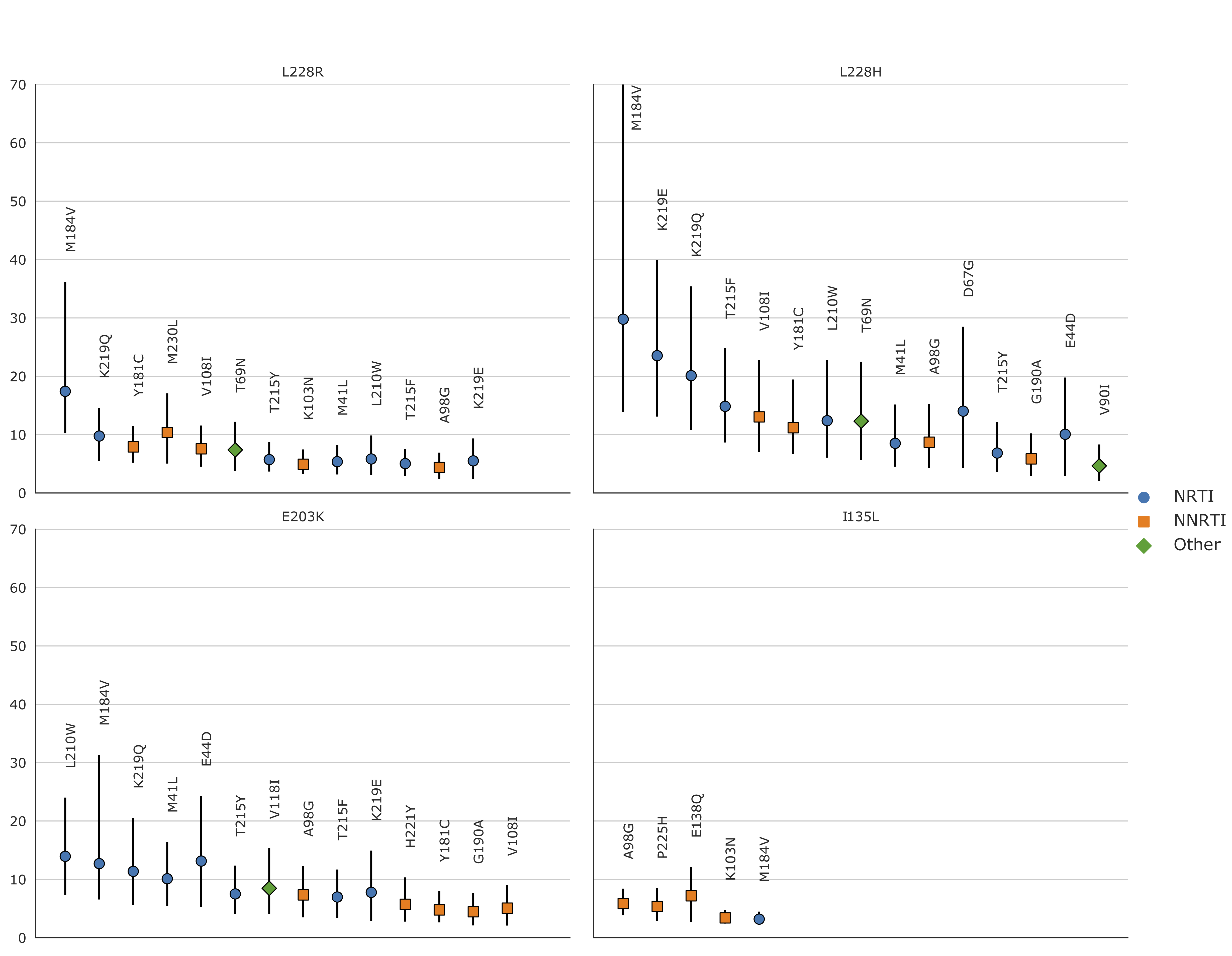
Figure C.1: Relative risks of the new mutations with regards to known RAMs on the African dataset
(i.e. the prevalence of the new mutation in sequences with a given RAM divided by the prevalence of the new mutation in sequences without the RAM). RRs were only computed for mutations (new and RAMs) that appeared in at least 30 sequences, which is why RRs were not computed for H208Y and D218E. 95% confidence intervals, represented by vertical bars, were computed with 1000 bootstrap samples of the African sequences. Only RRs with a lower CI boundary greater than 2 are shown. The shape and color of the point represents the type of RAM as defined by Stanford’s HIVDB. Blue circle: NRTI, orange square: NNRTI, green diamond: Other. For the RR of L228H with regards to M184V, the upper CI bound is infinite. The new RAMs have high RR values for known RAMs similar to those obtained on the UK dataset. We also arrive at similar conclusions, I135L being associated with NNRTIs, E203K and L228H to NRTI and L228R to both. RR values are shown from left to right, by order of decreasing values on the lower bound of the 95% CI.

C.3 S2 Fig.

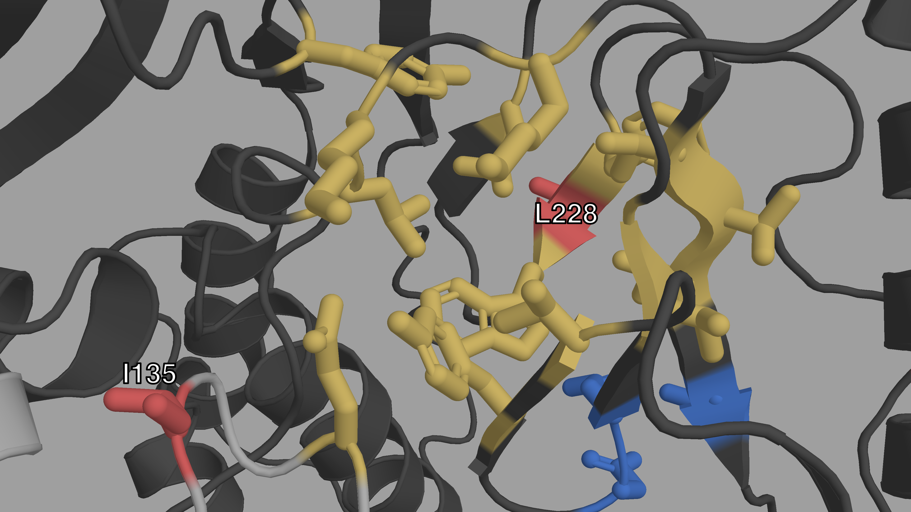
Figure C.2: Closeup structural view of the entrance of the NNIBP of HIV-1 RT
The p66 subunit is colored in dark gray, the p51 subunit in light gray. The NNIBP is highlighted in yellow. The active site is colored in blue. We can see the physical proximity of I135 (red) to the entrance of the NNIBP. We can also see how L228 (red) is between 2 AAs of the NNIBP.

C.4 S3 Fig.

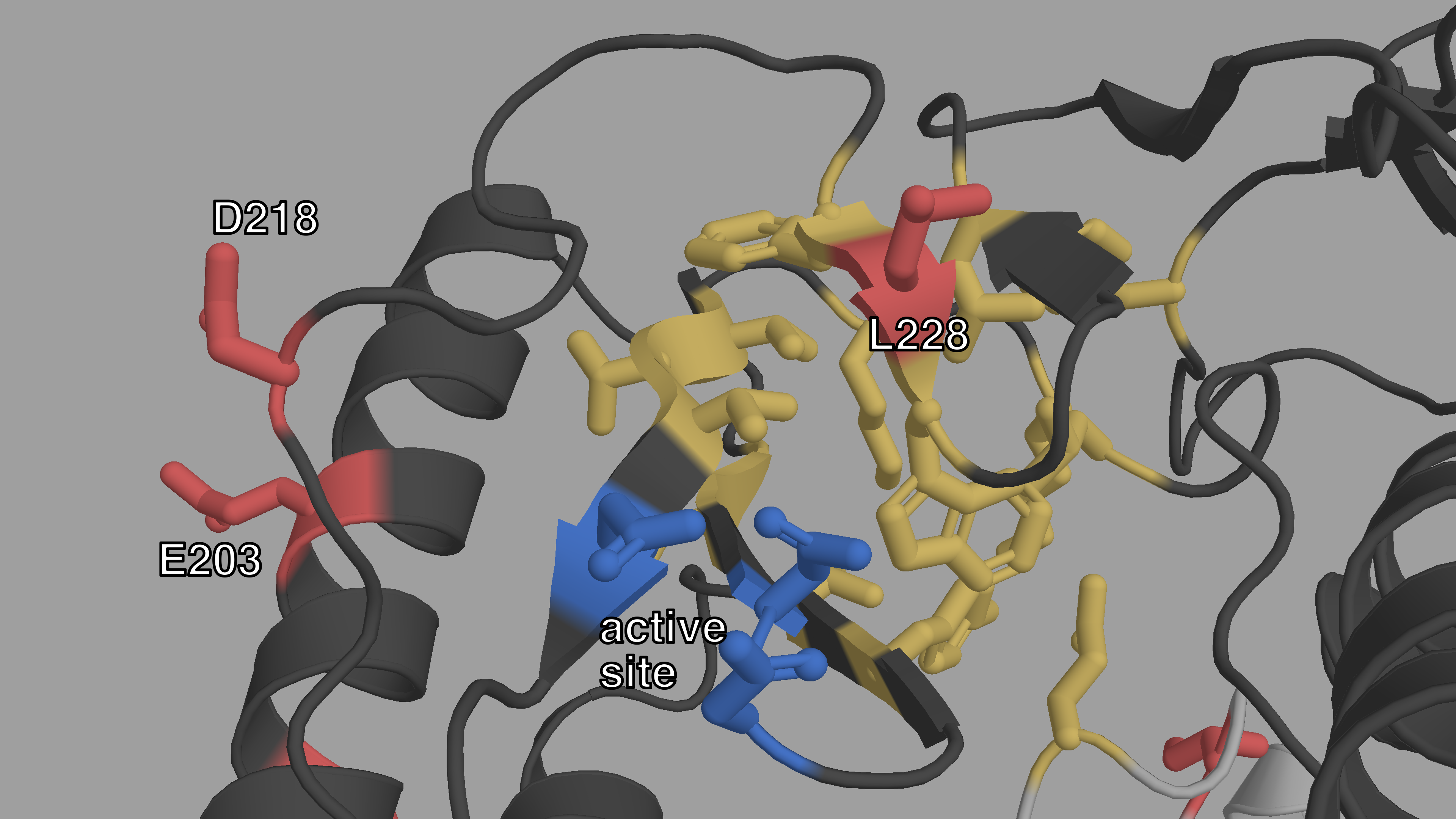
Figure C.3: Closeup structural view of the active site of HIV-1 RT.
The p66 subunit is colored in dark gray, the p51 subunit in light gray. The active site is highlighted in blue. The NNIBP is colored in yellow. L228, E203 and D218 (red) are also very close on either side of the active site.

C.5 S1 Table.

C.6 S2 Appendix. (Fisher exact tests)

Fisher exact tests on pairs of mutations. A detailed explanation of the procedure followed to test pairs of mutations for association with treatment. Detailed numerical results are also given.

In order to study epistasis further we conducted conducted Fisher exact tests between every pair of mutations in the UK dataset (\(n=867,903\)) and the treatment status, corrected the p-values with the Bonferroni method with an overall risk level \(\alpha=0.05\).
Out of these tests, \(1,309\) pairs were significantly associated with treatment status. \(424\) out of \(1,309\) these pairs were two known RAMs, \(806\) of these pairs contained one known RAM and only \(79\) tests had pairs involving no known RAM at all. Furthermore out of these \(1,309\) significantly associated pairs, \(829\) contained two mutations that were significantly associated to treatment when testing mutations one by one. In \(478\) pairs, one of the two mutations is associated to treatment on its own, and the remaining 2 pairs, none of the mutations were significantly associated with treatment on their own.
These 2 pairs were K103R + V179D and T165I + K173Q. The first pair, is a pair of known RAMs and this interaction is characterized in the HIVDb database (https://hivdb.stanford.edu/dr-summary/comments/NNRTI/). The second pair is made up of new mutations, and the corrected p-value is \(0.02\). In the Standford HIVDB, T165I has been associated to a reduction in EFV susceptibility.
Out of the \(1,309\) pairs significantly associated to treatment, \(151\) contained at least one of our 6 new potential RAMs, in \(6\) cases the pair was made up of 2 of them.
In the UK dataset, phylogenetic correlation is likely very impactful with regards to these tests. Indeed, the sequences are far from being independent. In order to alleviate this effect we decided to test the sigficative pairs again on the African dataset, and once more correct with the Bonferroni procedure.
Out of the \(1,309\) tests \(294\) have significative p-values after correction. Out of these \(221\) pairs were composed of 2 mutations individually significatively associated with treatment. The remaining \(73\) pairs had one mutation significantly associated with treatment.
Out of the \(221\) significative tests, 156 pairs were composed of 2 known RAMS while \(135\) had one known RAM in the pair. The remaining 3 pairs that do not contain a known RAM all contained either L228R or L228H which are both part of our 6 potential RAMS.

C.7 S1 Data.

Archive of figure generating data. A zip archive containing the processed data used to generate each panel of the main figures.

Download data

C.8 S2 Data.

List of known DRMs. A .csv file containing all the known RAMs used in this project as well as the corresponding feature name in the encoded datasets. Obtained from (hivdb.stanford.edu/dr-summary/comments/NRTI/) and (hivdb.stanford.edu/dr-summary/comments/NNRTI/).

Download data

References

150.

Vinh, N. X., Epps, J. & Bailey, J. Information Theoretic Measures for Clusterings Comparison: Variants, Properties, Normalization and Correction for Chance. Journal of Machine Learning Research 11, 18 (2010).

380.

Brodersen, K. H., Ong, C. S., Stephan, K. E. & Buhmann, J. M. The Balanced Accuracy and Its Posterior Distribution. in 2010 20th International Conference on Pattern Recognition 3121–3124 (2010). doi:10.1109/icpr.2010.764.

409.

McGinnis, W. et al. Scikit-Learn-Contrib/Categorical-Encoding: Release For Zenodo. (2018) doi:10.5281/zenodo.1157110.

410.

Kawashima, S. et al. AAindex: amino acid index database, progress report 2008. Nucleic Acids Res 36, D202–d205 (2008).

744.

Castresana, J. Selection of Conserved Blocks from Multiple Alignments for Their Use in Phylogenetic Analysis. Mol Biol Evol 17, 540–552 (2000).

745.

Pedregosa, F. et al. Scikit-learn: Machine Learning in Python. Journal of Machine Learning Research 12, 2825–2830 (2011).

746.

Virtanen, P. et al. SciPy 1.0: Fundamental algorithms for scientific computing in Python. Nature Methods 17, 261–272 (2020).

747.

Seabold, Skipper & Perktold, Josef. Statsmodels: Econometric and Statistical Modeling with Python. in Proceedings of the 9th Python in Science Conference (eds. Walt, Stéfan van der & Millman, Jarrod) 92–96 (2010). doi:10.25080/Majora-92bf1922-011.

748.

Vinh, N. X. & Epps, J. A Novel Approach for Automatic Number of Clusters Detection in Microarray Data Based on Consensus Clustering. in 2009 Ninth IEEE International Conference on Bioinformatics and BioEngineering 84–91 (2009). doi:10.1109/bibe.2009.19.

749.

Harremoes, P. Mutual information of contingency tables and related inequalities. in 2014 IEEE International Symposium on Information Theory 2474–2478 (Ieee, 2014). doi:10.1109/isit.2014.6875279.